Tensorflow 2.0搭建ResNet网络 -- CIFAR-10数据集
这篇教程我们来实现Kaiming He大神提出的ResNet网络,并在CIFAR-10数据及上进行测试,我的测试结果完全复现了论文中的精度。本文中的参数设置、数据增强等内容均遵循原文。
网络搭建
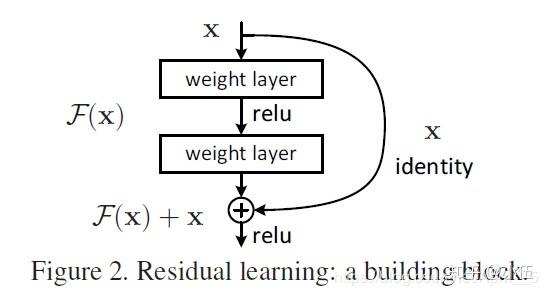
ResNet原文: Deep Residual Learning for Image Recognition 这篇文章中提出了像下面这样的经典残差结构。
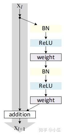
后续Kaiming He又对这一结构进一步研究改进(Identity Mappings in Deep Residual Networks),给出了Batch normalization和Relu的最佳应用位置。
不难理解,在ResNet中网络不再是只有一条道路,而是会有分支,因此model.add()并不适用,我们需要实例化各个层,然后指定其输入输出,首先我们要实现一个生成残差块的函数
def residual_block(inputs, channels, strides=(1, 1)):
    net = BatchNormalization(momentum=0.9, epsilon=1e-5)(inputs)
    net = Activation('relu')(net)

    if strides == (1, 1):
        shortcut = inputs
    else:
        shortcut = Conv2D(channels, (1, 1), strides=strides)(net)

    net = Conv2D(channels, (3, 3), padding='same', strides=strides)(net)
    net = BatchNormalization(momentum=0.9, epsilon=1e-5)(net)
    net = Activation('relu')(net)
    net = Conv2D(channels, (3, 3), padding='same')(net)

    net = add([net, shortcut])
    return net
这里我们需要注意,当取strides=(2, 2)压缩特征图大小时,数据的通道数会加倍,此时shortcut无法直接与卷积后的结果相加,需要采用1*1的卷积进行线性变换,增加通道数。
有了生成残差块的函数后,就能简洁的生成整个ResNet模型。
def ResNet(inputs):
net = Conv2D(16, (3, 3), padding='same')(inputs)
for i in range(stack_n):
net = residual_block(net, 16)
net = residual_block(net, 32, strides=(2, 2))
for i in range(stack_n - 1):
net = residual_block(net, 32)
net = residual_block(net, 64, strides=(2, 2))
for i in range(stack_n - 1):
net = residual_block(net, 64)
net = BatchNormalization(momentum=0.9, epsilon=1e-5)(net)
net = Activation('relu')(net)
net = AveragePooling2D(8, 8)(net)
net = Flatten()(net)
net = Dense(10, activation='softmax')(net)
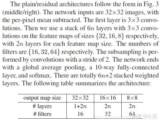
return net这里的网络配置与常见的ResNet稍有不同,是针对CIFAR-10所设计的结构,位于原文第七页左栏。
最后,再指定网络的整体的输入和输出。
img_input = Input(shape=(32, 32, 3))
output = ResNet(img_input)
model = models.Model(img_input, output)
以(224, 224)大小的图像为输入的经典ResNet可以在这里找到
https://github.com/Apm5/tensorflow_2.0_tutorial/blob/master/CNN/ResNet.py
数据增强
首先加载Cifar-10数据可以使用tensorflow中提供的官方加载函数
(train_images, train_labels), (test_images, test_labels) = tf.keras.datasets.cifar10.load_data()
train_labels = tf.keras.utils.to_categorical(train_labels, 10)
test_labels = tf.keras.utils.to_categorical(test_labels, 10)
也可以将事先将数据下载到本地,然后使用我提供的加载函数
(train_images, train_labels, test_images, test_labels) = load_CIFAR('/home/user/Documents/dataset/Cifar-10')对于数据增强要说明的是,tensorflow对数据增强原本是有一个非常好用的库
from tensorflow.keras.preprocessing.image import ImageDataGenerator但是在2.0正式版中,这个库和对应的训练方法model.fit_generator()出了问题,训练的耗时增加了3-4倍。tensorflow的官方人员给出的答复是这确实是一个bug(issue #33177),并且他们决定弃用这个方法而不是修复。给出的解决办法是直接用model.fit()接收ImageDataGenerator生成的数据,但这又产生了一个额外的问题,在每个epoch之前程序提示'Filling up shuffle buffer (this may take a while)’ 这也是一份很可观的额外时间开销,对cifar来说我的机器需要10s,每个epoch多10s是不能接受的,所以不得不采用其他的库完成数据增强,我这里采用cv2。
仍然是按照原文的设定,所有图像首先在R、G、B通道分别进行归一化处理。
def color_normalize(train_images, test_images):
    mean = [np.mean(train_images[:, :, :, i]) for i in range(3)]  # [125.307, 122.95, 113.865]
    std = [np.std(train_images[:, :, :, i]) for i in range(3)]  # [62.9932, 62.0887, 66.7048]
    for i in range(3):
        train_images[:, :, :, i] = (train_images[:, :, :, i] - mean[i]) / std[i]
        test_images[:, :, :, i] = (test_images[:, :, :, i] - mean[i]) / std[i]
    return train_images, test_images
需要注意测试数据不应参与均值和方差的计算。 然后在训练时,每张图片首先在四周各填充4像素,将图像增大到40 40,然后随机选择32 32的区域,并随机左右翻转。
def images_augment(images):
    output = []
    for img in images:
        img = cv2.copyMakeBorder(img, 4, 4, 4, 4, cv2.BORDER_CONSTANT, value=[0, 0, 0])
        x = np.random.randint(0, 8)
        y = np.random.randint(0, 8)
        if np.random.randint(0, 2):
            img = cv2.flip(img, 1)
        output.append(img[x: x+32, y:y+32, :])
    return np.ascontiguousarray(output, dtype=np.float32)
对于测试数据,直接输入原图像即可。
训练与测试
由于model.fit对数据增强也不适用了,所以我们需要自己实现训练的各个细节,也是对网络有深入的了解。 首先是设定变学习率
batch_size = 128
train_num = 50000
iterations_per_epoch = int(train_num / batch_size)
learning_rate = [0.1, 0.01, 0.001]
boundaries = [80 * iterations_per_epoch, 120 * iterations_per_epoch]
learning_rate_schedules = optimizers.schedules.PiecewiseConstantDecay(boundaries, learning_rate)
optimizer = optimizers.SGD(learning_rate=learning_rate_schedules, momentum=0.9, nesterov=True)learning_rate和boundaries的设置结果是让网络在前80轮学习率0.1,80到120轮学习率0.01,后续为0.001直到结束。
然后设置损失函数,包括交叉熵和l2 loss两部分。
def cross_entropy(y_true, y_pred):
    cross_entropy = -tf.reduce_sum(y_true * tf.math.log(tf.clip_by_value(y_pred, 1e-7, 1.0 - 1e-7)), axis=-1)
    return tf.reduce_mean(cross_entropy)

def l2_loss(model, weights=weight_decay):
    variable_list = []
    for v in model.trainable_variables:
        if 'kernel' or 'bias' in v.name:
            variable_list.append(tf.nn.l2_loss(v))
    return tf.add_n(variable_list) * weight
然后自己定义每个iteration的网络正向计算和梯度更新
@tf.function
def train_step(model, optimizer, x, y):
    with tf.GradientTape() as tape:
        prediction = model(x, training=True)
        ce = cross_entropy(y, prediction)
        l2 = l2_loss(model)
        loss = ce + l2
        gradients = tape.gradient(loss, model.trainable_variables)
    optimizer.apply_gradients(zip(gradients, model.trainable_variables))
return ce, prediction函数前的@tf.function修饰非常重要,由于tensorflow2.0默认为动态图,@tf.function能让网络转为静态图,极大优化性能,加快运算速度。因此,在调试网络时,可以注释掉@tf.function然后直接print打印出希望查看的变量值,测试结束后反注释@tf.function即可。
测试部分则无需更新梯度,只计算结果即可。model中的training参数是配置一些在训练和测试时有不同表现的层(常见的是dropout和batch normalization)
@tf.function
def test_step(model, x, y):
    prediction = model(x, training=False)
    ce = cross_entropy(y, prediction)
    return ce, prediction
至此,网络的所有细节均已完成,再完成对网络输出的准确率统计、交叉熵统计即可。需要注意测试时理论上是不存在batch的概念的,但为了测试速度,通常仍采用和训练时类似的办法输入一批数据。
def train(model, optimizer, images, labels):
    sum_loss = 0
    sum_accuracy = 0

    # random shuffle
    seed = np.random.randint(0, 65536)
    np.random.seed(seed)
    np.random.shuffle(images)
    np.random.seed(seed)
    np.random.shuffle(labels)

    for i in tqdm(range(iterations_per_epoch)):
        x = images[i * batch_size: (i + 1) * batch_size, :, :, :]
        y = labels[i * batch_size: (i + 1) * batch_size, :]
        x = images_augment(x)

        loss, prediction = train_step(model, optimizer, x, y)
        sum_loss += loss
        sum_accuracy += accuracy(y, prediction)

    print('epoch:%d, ce_loss:%f, l2_loss:%f, accuracy:%f' %
          (epoch, sum_loss / iterations_per_epoch, l2_loss(model), sum_accuracy / iterations_per_epoch))

def test(model, images, labels):
    sum_loss = 0
    sum_accuracy = 0

    for i in tqdm(range(test_iterations)):
        x = images[i * test_batch_size: (i + 1) * test_batch_size, :, :, :]
        y = labels[i * test_batch_size: (i + 1) * test_batch_size, :]

        loss, prediction = test_step(model, x, y)
        sum_loss += loss
        sum_accuracy += accuracy(y, prediction)

    print('test, loss:%f, accuracy:%f' %
(sum_loss / test_iterations, sum_accuracy / test_iterations))tqdm是个很好用的进度条,推荐多多了解。
最后在stack_n取3的时候测试集准确率约91.5%,stack_n取18的时候测试集准确率约94.0%,甚至比原文还高了一点点。
完整的代码可以在我的github上找到
ResNet for CIFAR
https://github.com/Apm5/tensorflow_2.0_tutorial/blob/master/CNN/ResNet_CIFAR.py
ResNet
https://github.com/Apm5/tensorflow_2.0_tutorial/blob/master/CNN/ResNet.py
评论列表(0条)